Table of Contents
i. Calculation of Gasoline Per Capita Consumption (GPC) ————————- 3
ii. Signs of Regression Coefficient with Economic Theory and Reasoning ——- 6
iii. Simple Regression Model ———————————————————- 7
iv. Re-run Regression Equation ——————————————————- 9
v. Recommendations for the Energy Firm ——————————————- 10
References ——————————————————————————- 11
i. Calculation of Gasoline Per Capita Consumption (GPC)
The complete computation of Gasoline per Capital Consumption can be found in the attached excel sheet. Table-1 shows the output while Figure-1 below is showing the trend behind the same.
GPC = (1,000,000 * GasExp) / (Pop * Gasp) —— (1)


The trend from the graph is clear as the trend of Gasoline Consumption is positive as it has been increasing with each of the passing years. However, the magnitude of such an increase was rapid from the year 1953 till 1979, and then the increment was steady from 1979 till the very end of 2003, as found in the diagram mentioned above. In other words, the consumption of Gasoline has been increasing with time.
ii. Signs of Regression Coefficient with Economic Theory and Reasoning
The equation is as follows;
logGPC = logA+ B1 log PG + B2 log Y + B3 log PNC + B4 log PUC
The log here is showing the difference in the values in the current year compared to the preceding year. In other words, “Log” is about change in the values. “A” is referred to as “Alpha” here which is a constant value that comes over the screen when multiple or regression model is applied. Since this value is constant, therefore it can be changed with any changes in other values. B1, B2, B3 and B4 are referred to as “Beta” which are the values that can be changed or these are the independent variables. Any change in these values will be impacting on the dependent variable which is GPC. The terms mentioned with each of the betas are their literal meanings as follows;
- PG = Gasoline Price
- Y = Per Capita Income
- PNC = Price of New Cars
- PUC = Price of Used Cars
The main reasoning behind the inclusion of the above-mentioned independent variables on the dependent one is to evaluate its connection with the GPC.
iii. Simple Regression Model
Table-2 is showing the regression output
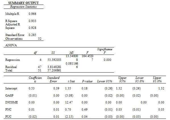
From the chart mentioned above, it is clear that the relationship between the variables is significant. The Coefficients attached to the dependent variable such as GPC are positive and direct. It means that when the income increases, the Gasoline consumption per capita also increases. It is also found that when Gasoline Consumption per capita increases, the price of new cars also increases. However, the relationship between GASP and GPC is negative. It means that when the price index of Gasoline increases, the Gasoline consumption per capita decreases. The regression result found in the table mentioned above is the same as found in the economic theory. As mentioned by Fukase&Martin (2020), the Income of an individual is directly connected with consumption. The researcher mentioned that when income increases the propensity of consumption also increases considerably. The same is associated with this particular field as well.
GPC = logA+ B1 log PG + B2 log Y + B3 log PNC + B4 log PUC
GPC = 0.53 + (-0.01) + (0.000334) + (0.01) + (-0.02)
GPC = 0.51 or 51%
It means that any increase or decrease in the variables in the equation will be having a definite impact on the Per capita Consumption of Gasoline.
iv. Re-run Regression Equation
log GPC = logA+B1 log PG+B2 log Y +B3 log PNC+B4 log PUC+B5 log PrevGPC
= 0.53 + (-0.01) + (0.000334) + (0.01) + (-0.02) + (0.51)
GPC = 1.02 or 102%
Long run Elasticity
= 0.51 / (1 – 1.02)
= 0.51/0.02 = 25
Based on the same estimates, it can be said that the elasticity in these variables is positive, and it is showing that the single dollar change in the Gasoline Price changes the consumption per capita by 25%.
v. Recommendations for the Energy Firm
Based on the regression output, a positive connection is found between the income of the individuals in the United States and its impact on Gasoline Consumption. Therefore, Energy Firms should consider those states of the country which have high median income compared to other states such as Maryland, New Jersey, Mississippi and others (Chien, Zhang&Hsu, 2021). Since, the Median income of the people is comparatively higher than in other states of the United States of America that ultimately translated to higher consumption of Gasoline, which will be effective for maximizing the financial benefits of the company. Similarly, the Energy firms could see the cities or the states with the highest number of new cars buying which has a strong connection with Gasoline Consumption because it uses for travelling purposes.
References
Chien, F., Zhang, Y., & Hsu, C. C. (2021). Assessing the nexus between financial development and energy finance through demand-and supply-oriented physical disruption in crude oil. Environmental Science and Pollution Research, 28, 66086-66100.
Fukase, E., & Martin, W. (2020). Economic growth, convergence, and world food demand and supply. World Development, 132, 104954.
Please place the order on the website to get your own firstly economicsassignmentshelp.com result.
Related Samples